EM Algorithm for Linear Clusters

Here is an interesting situation occurred to me. In a scatter plot, it is clear that there are two straight lines and each line is contanminated by some noise. Then it is interesting to find the slopes of the line and cluster the points. Since the original data is classified, let’s do some simple toy test. Here I generate a toy example:

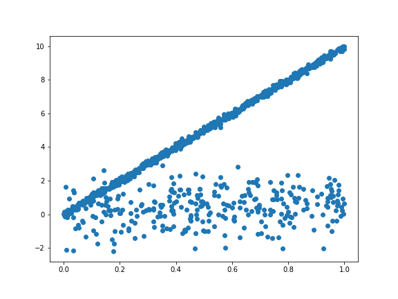
X = np.random.uniform(0,1,size= 1000)
y = np.concatenate( (X[:700]*10.0+ np.random.normal(0.0,0.1, size=700),
                     X[700:]*1.0 + np.random.normal(0.0,1.0, size=300)))
plt.scatter(X,y)
plt.show()

In this problem, we have two hidden linear models with slope as $10$ and $1$ respectively. Besides, the variance for the model is quite different, one is $0.1$ and the other is $1$. Thus we need to cluster the points to the corresponding linear model and get the parameters. This motivates me to write an EM algorithm for linear clusters.

The EM Algorithm for Linear Clusters:

The model:

data are from some line clusters. The total number clusters is given as $C$. The data is given as $(\mathbf{x}_i, y_i)$ and there is a hidden variabe $z_i$ indicating which cluster the data is drawn from. Then the data obey the distribution.

\[P(\mathbf{x}_i,y_i | z_i = z) = \frac{1}{\sqrt{2\pi\sigma_z^2}} \exp\left(-\frac{(y_i-\mathbf{x}_i\beta_z)^2}{2\sigma_z^2} \right)\]

for slope vector $\beta_z$. Also, the prior distribution of $z_i$ is given as

\[P(z_i = z) = \alpha_z\]

The problem the contains the parameters $\theta = {\alpha_z, \beta_z, \sigma_z^2} $ for $z = 1,\cdots C$.

The EM algorithm for this model:

If we are given the parameters $\theta_n$ at a given iteration $n$. Then the EM algorithm says:

\[\theta_{n+1} = \arg\max_{\theta} \sum_{i=1}^N \sum_{z_i=1}^C p(z_i|\mathbf{x}_i,y_i,\theta_n) \left( \log(\alpha_{z_i}) -\frac{1}{2}\log \sigma_{z_i}^2 - \frac{(y_i-\mathbf{x}_i\beta_{z_i})^2 }{2\sigma_{z_i}^2} \right)\]

Note the factor $p(z_i = z \vert x_i,y_i,\theta_n)$ is fixed in this step and it simply assigns the point $\mathbf{x}_i,y_i$ to a specific cluster. We simplify the notation as $p(z_i=z) = p(z_i = z\vert x_i,y_i,\theta_n)$. We also need to optimize subject to the constraint that $\sum_c \alpha_c = 1$. Thus, the function becomes

\[l(\theta) = \sum_{i=1}^N \sum_{z=1}^C p(z_i = z )\left( \log(\alpha_{z}) -\frac{1}{2}\log \sigma_{z}^2 - \frac{(y_i-\mathbf{x}_i\beta_{z})^2 }{2\sigma_{z}^2} \right) - \lambda \sum_{c=1}^C \alpha_c\]

The fixed factor

\[p(z_i = z | x_i, y_i,\theta) = \frac{1}{Z}{\alpha_z \frac{1}{\sqrt{2\pi\sigma_z^2}} \exp(-\frac{(y_i-x_i\beta)^2}{2\sigma_z^2}) }\]

with $Z$ acts as the normalization

\[Z = \sum_{z=1}^C {\alpha_z \frac{1}{\sqrt{2\pi\sigma_z^2}} \exp(-\frac{(y_i-x_i\beta)^2}{2\sigma_z^2}) }\]

Optimization for $\alpha_c$

We first take the derivative with $\alpha_c$ for a specific cluster $c$.

\[\frac{d}{d\alpha_c} l(\theta) = \sum_{i=1}^N p(z_i=c) \frac{1}{\alpha_c} - \lambda = 0 \quad \Rightarrow \alpha_c = \frac{1}{\lambda}\sum_{i=1}^N{p(z_i = c)}\]

Because the $\alpha_c$ is normalized to $1$, the $\lambda$ acts as a normalization factor and thus,

\[\alpha_c = \frac{\sum_{i=1}^N p(z_i = c)}{\sum_{c=1}^C \sum_{i=1}^N p(z_i= c)}\]

Optimization for $\beta_c$

Take the derivative with $\beta_c$, we get

\[\frac{d}{d \beta_c} = \sum_{i=1}^N p(z_i = c) \frac{(y_i - \mathbf{x}_i\beta_z)\mathbf{x}^T_i}{\sigma_c^2} = 0\]

This indicates that

\[\beta_z = \left(\sum_{i=1}^N p(z_i=c) \mathbf{x}_i^T \mathbf{x}_i \right)^{-1} \left(\sum_{i=1}^N p(z_i = c) y_i \mathbf{x}_i^T \right)\]

If we stack $\mathbf{x}_i$ onto the matrix $X$ with $N\times p$ dimensions, i.e., each row is a sample $\mathbf{x}_i$, and if we define the diagonal $N\times N$ matrix, $P_c = \text{diag}(p(z_1=c),\dots p(z_N = c))$ , we could rewrite the $\beta_c$ as

\[\beta_c = (X^T P_c X)^{-1} X^T (P_c y)\]

Optimization for $\sigma_c$

Take the derivative with $\sigma_c$ , we get

\[\frac{d}{d\sigma_c} l(\theta) = -\frac{1}{2} \frac{1}{\sigma_c^2}\sum_{i=1}^N p(z_i =c) + \frac{1}{2(\sigma_c^2)^2}\sum_{i=1}^N p(z_i =c) (y_i-\mathbf{x}_i\beta_c)^2 = 0\]

This shows that

\[\sigma_c^2 = \frac{\sum_{i=1}^N p(z_i = c)(y_i-\mathbf{x}_i\beta_c)^2}{\sum_{i=1}^N p(z_i = c)}\]

Implement in Python:

We want to implement the above algorithm as an sklearn style class. We first construct the structure. In the initializer, we set up some variables for the optimization iterations. We aslo give the model freedom to take user specified initial $\beta$.

class LinearClustering(object):
    
	def __init__(self, n_clusters, initial_betas = None, 
				with_intercept = False, max_itr = 100, atol = 1e-6):
		
		self.C = n_clusters
        self.with_intercept = with_intercept
        self.max_itr = max_itr
        self.atol = atol
        self.alphas = np.array([1.0/self.C]*self.C)
        self.sigmas = np.array([1.0]*self.C)
        self.betas = None
        if initial_betas is not None:
            self.betas = np.array(initial_betas)

	def fit(self, X,y):

		pass

	def predict(self, X,y):

		pass

The main part is to implement the fit algorithm. We first set up the inputs correctly in numpy :

def fit(self, X,y):
    X = np.array(X)
    y = np.array(y)
    if len(X.shape) == 1 :
        X = X[:,None]
    if self.with_intercept:
        X = np.hstack( (np.ones( (X.shape[0],1)) , X ) )
    if self.betas is None:
        self.betas = np.random.normal(0,1,size=(self.C, X.shape[1]))

In the optimization algorithm, we need to first calulcate the probability $p({z_i}=z) = p(z_i = z|x_i,y_i,\theta_n)$. Here, we set up diffs as $N\times C$ matrix with row $i$ and column $j$ indicates the $(y_i-X_i\beta_j)^2$ in the line cluster $j$. The broadcasting in y[:,None] is to broadcast y to each rows instead of columns (python broadcasts from the last dimension). Then we update alphas by the previous calculation.

def fit(self, X,y): 
    # previous codes...
    it = 0
    err = None 
    while it < self.max_itr :   
        diffs = (y[:,None] - X.dot(self.betas.T))**2  # N*C
        pz = np.exp(-0.5*diffs/self.sigmas)/np.sqrt(2*np.pi*self.sigmas)*self.alphas #N*C
        pz = pz/np.sum(pz, axis=1, keepdims=True)
        self.alphas = np.sum(pz, axis = 0)
        self.alphas = self.alphas/np.sum(self.alphas)

By the similar logic, we update $\beta_c$ for each cluster c. With the updated new $\beta_c$, we can estimate the variance of the linear model $\sigma_c^2$.

def fit(self, X,y):
    # previous codes ....
    # in the while loop: 
    while it < self.max_itr :
        # ...
        for c in range(self.C):
            M = X.T.dot(X*pz[:,c,None])
            self.betas[c,:] = np.linalg.solve(M,X.T.dot(y*pz[:,c])) 
        diffs = (y[:,None] - X.dot(self.betas.T))**2  #N*C
        self.sigmas = np.sum(pz*diffs, axis = 0)/np.sum(pz, axis = 0)

Then we completed the main part of the algorithm. we just need to give some conditions for it to stop. Here, I choose to use the two norms of $\beta$. I averaged the two norms of the change of $\beta$ over the clusters. Below is the complete code for the fit function. Here I modified the code a little bit so that the calculation for diffs will occur once for each iteration. Also, I calculatd log pz first and subtract leading terms and this will make the calculation stable.

def fit(self, X,y):
    X = np.array(X)
    y = np.array(y)
    if len(X.shape) == 1 :
        X = X[:,None]
    if self.with_intercept:
        X = np.hstack( (np.ones((X.shape[0],1)), X ) )
    if self.betas is None:
        self.betas = np.random.normal(0,1,size=(self.C, X.shape[1]))

    it = 0
    err = None
    diffs = (y[:,None] - X.dot(self.betas.T))**2  # N*C # put the diffs here to avoid calculating it twice
    while it < self.max_itr :
        logpz = -0.5*diffs/self.sigmas - 0.5*np.log(2*np.pi*self.sigmas) + np.log(self.alphas) #N*C
        logpz_reg = logpz - np.max(logpz, axis = -1, keepdims = True) 
        pz = np.exp(logpz_reg)
        pz = pz/np.sum(pz, axis=1, keepdims=True)
        self.alphas = np.sum(pz, axis = 0)
        self.alphas = self.alphas/np.sum(self.alphas)
        old_betas = np.copy(self.betas)
        for c in range(self.C):
            M = X.T.dot(X*pz[:,c,None])
            self.betas[c,:] = np.linalg.solve(M,X.T.dot(y*pz[:,c]))
        diffs = (y[:,None] - X.dot(self.betas.T))**2  #N*C
        self.sigmas = np.sum(pz*diffs, axis = 0)/np.sum(pz, axis = 0)
        err = np.mean(np.sqrt(np.sum((self.betas - old_betas)**2, axis=1)) )
        if err < 0.8* self.atol:
            print (it, err)
            break
        it+=1

    return self

The prediction function should be striaght forward and below is the code.

def predict(self, X, y ):
    X = np.array(X)
    y = np.array(y)
    if len(X.shape) == 1 :
        X = X[:,None]
    if self.with_intercept:
        X = np.hstack( (np.ones( (X.shape[0],1) ), X ) )
    diffs = 0.5*(y[:,None] - X.dot(self.betas.T))**2 
    pz = np.exp(-diffs/self.sigmas)/np.sqrt(2*np.pi*self.sigmas)*self.alphas 
    return np.argmax(pz, axis=1).ravel()

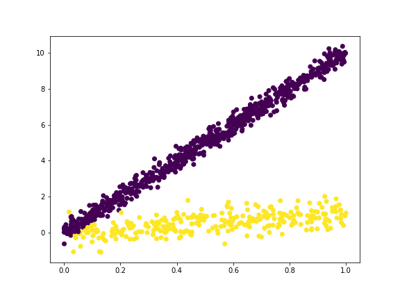
It worths to try our model on the raw data to see whether we can calssify it out

linearC = LinearClustering(n_clusters = 2)
linearC = linearC.fit(X , y)
clas = linearC.predict(X,y)
plt.scatter(X,y,c = clas)
plt.show()

It is also worths to check out parameter estimation:

print ("alphas", linearC.alphas)
print ("sigmas", linearC.sigmas)
print ("beta1", linearC.betas[0])
print ("beta2", linearC.betas[1])

alphas [0.30178798 0.69821202]
sigmas [0.99119916 0.01048012]
beta1 [0.76533822]
beta2 [9.99494678]

This estimation is pretty good except that because the variance for the slope $1$ cluster is too large, the slope estimation is not that good. This effect is worse when we only have 30 percent of the data points are from that cluster.

If we play with it by setting the line with slope $10$ to have $\sigma^2= 0.3^2$ and the the line with slope $1$ to have $\sigma^2 = 0.5^2$, we will see that

and the outputs as

alphas [0.70387515 0.29612485]
sigmas [0.0943882  0.19680254]
beta1 [9.98451242]
beta2 [1.05238964]

which is quite close to the hidden parameters.

Some Comments

Althogh this works for this simple toy problem, it is not guaranteed to converge well on an arbitrary dataset. This heavily depends on the initialization. Also, this algorithm is not the only possible one. Here we use the $y$ distance to model the relation between points and the hidden lienar line. We could also use “point to line distance” to preserve the symmetry between $x$, $y$. If I have time in the future, will try for that model.