
Realized Garch model with dynamical conditional correlation
The accompanying report is here
The package rGARCH_DCC is included here and it is priliminary and hopefully I can make it user friendly and will publish to my github.
Realized GARCH-DCC Model
In this project we will study the realized GARCH-DCC model. This model is designed to do forecast of volatility and correlation among symbols. The model takes into high frequency data.
Specifically, we let $r^i_t$ to denote the log return $\log P^i_t - \log P^i_{t-1}$ for stock $i$, $\sigma^i_t$ to be the conditional variance of stock $i$, $z_t^i$ to be the shock for stock $i$ and $C_t$ be the conditional correlation matrix among $z_t^i$. The model can be described as
\[\begin{aligned} &r_t^i = \mu^i + \sigma_t^i z_t^i \\ &\log(\text{RV}_t^i) = \xi^i + \phi^i \log(\sigma_{t}^i)^2 + \tau^i_1 z_t^i + \tau^i_2 ((z_t^i)^2-1) + u_t^i\\ &(\sigma_{t+1}^i)^2 = \omega^i + \beta^i (\sigma_{t}^i)^2 + \gamma^i \text{RV}_t^i \\ &C_t = \text{diag}(Q_t)^{-1/2} Q_t \text{diag}(Q_t)^{-1/2} \label{eq:section2:normalization} \\ &Q_{t+1} = S(1-a-b) + a (z_t z_t^T) + bQ_t \label{eq:section2:covariance} \\ &z_t \sim \mathcal{N}(0, C_t) \\ &u_t \sim \mathcal{N}(0, \Sigma_u) . \end{aligned}\]The first equation describes the return using the volatility scale and the constant expected mean $\mu^i$. The second equation describes the “measurement” mechanics: the realized variance depends on the hidden true volatility and the shocks as well as a measurement noise $u_t$. These $u_t$ have zero pairwise correlation but have different scales for different stock $i$ and thus $\Sigma_u$ is a diagonal matrix. The log transformation on the measurement equation is to make the noise $u_t$ similar to Normal distribution. The third equation is the updating equation for the volatility $\sigma_t^i$. Notice, the usual GARCH model uses return squared to update the volatility but here, we use the more accurate estimate, the realized variance. The $Q_{t}$ is the sample estimate of the conditional covariance matrix of $z_t$ and the update equation is mean revert to the sample estimation $S$. The normalization ensures that the covariance matrix for the shocks is normalized.
import numpy as np
import pandas as pd
import pandas_market_calendars as mcal
import datetime

from scipy.optimize import minimize
from sklearn.linear_model import LinearRegression
from arch import arch_model

import matplotlib.pyplot as plt
from matplotlib.ticker import MaxNLocator
import matplotlib.dates as mdates
from matplotlib.ticker import FormatStrFormatter
from statsmodels.graphics.gofplots import qqplot
import matplotlib

from rGARCH_DCC import *


font = { "family": "sans",
         "weight": "normal",
         'size'  : 12}

matplotlib.rc('font', **font)
Load Data
We first load data from https://firstratedata.com/free-intraday-data. The data contains AAPL, AMZN, FB, MSFT, TSLA and SP500 one minute tick data in 2019.
FOLDER = "/Users/bunny_home/Documents/Cunwei/stockData/"
AAPL_FILE = FOLDER + "AAPL_FirstRateDatacom1.txt"
AMZN_FILE = FOLDER + "AMZN_FirstRateDatacom1.txt"
FB_FILE   = FOLDER + "FB_FirstRateDatacom1.txt"
MSFT_FILE = FOLDER + "MSFT_FirstRateDatacom1.txt"
TSLA_FILE = FOLDER + "TSLA_FirstRateDatacom1.txt"
SPX_FILE  = FOLDER + "SPX_Firstratedata1.txt"

FILES = {"AAPL" : AAPL_FILE,
         "AMZN" : AMZN_FILE,
         "FB"   : FB_FILE,
         "MSFT" : MSFT_FILE,
         "TSLA" : TSLA_FILE,
         "SP500": SPX_FILE}
Since there are missing ticks in the data, we then construct time ticks frame in one minute frequency and left join with the data. This ensures the data all in one tick frequency and can be joined conveniently.
def get_trading_index(start, end):
    nyse = mcal.get_calendar('NYSE')
    days = nyse.valid_days(start_date = start, end_date = end)
    date_index = []

    for d in days:
        #print (d)
        early_close = [datetime.date(d.year, 7,3),
                   datetime.date(d.year, 11,29),
                   datetime.date(d.year, 12,24)]
        if d.date() in early_close :
            open_time = pd.Timestamp(year=d.year, month = d.month,
                                     day = d.day, hour = 9, minute = 30)
            close_time = pd.Timestamp(year=d.year, month = d.month,
                                      day = d.day, hour = 13, minute = 0)
        else:
            schedule = nyse.schedule(start_date = d.date(), end_date = d.date(), tz = nyse.tz.zone)
            open_time = schedule["market_open"][0].replace(tzinfo=None)
            close_time = schedule["market_close"][0].replace(tzinfo=None)

        date_index += pd.date_range(open_time, close_time, freq = "1T")

    return pd.Series(date_index)


def load_file(filename, trading_index):
    df = pd.read_csv(filename, header=None)
    df.columns = ["time", "open", "high", "low", "close", "volume"][:len(df.columns)]
    df["time"] = pd.to_datetime(df["time"], format= "%Y-%m-%d %H:%M:%S")
    df = df.set_index("time")

    dummy = pd.DataFrame.from_dict({"time":trading_index,
                                    "dummy": np.ones(len(trading_index)) } )
    dummy = dummy.set_index("time")

    df = dummy.join(df)
    df = df.drop("dummy", axis = 1)
    return df
DATA = {}
print ("Generating time ticks ...")
TRADING_MINUTES = get_trading_index("2019-01-01", "2019-12-30")
print ("Ticks number: %d" % (len(TRADING_MINUTES)))
for F in FILES:
    data = load_file(FILES[F], TRADING_MINUTES)
    DATA[F] = data
    print ("%s\t length: %d, done" %(F, data.shape[0]))
Generating time ticks ...
Ticks number: 97601
AAPL	 length: 97601, done
AMZN	 length: 97601, done
FB	 length: 97601, done
MSFT	 length: 97601, done
TSLA	 length: 97601, done
SP500	 length: 97601, done
combine = []
keys = []
for s in DATA:
    combine.append(DATA[s]["close"])
    keys.append(s)
prices = pd.concat(combine, axis = 1, keys = keys)
prices
| AAPL | AMZN | FB | MSFT | TSLA | SP500 | |
|---|---|---|---|---|---|---|
| time | ||||||
| 2019-01-02 09:30:00 | 154.7800 | 1466.9690 | 129.7950 | 99.010 | 305.9600 | 2470.40 |
| 2019-01-02 09:31:00 | 155.1597 | 1469.0000 | 130.1100 | 99.250 | 308.8050 | 2470.80 |
| 2019-01-02 09:32:00 | 154.8073 | 1470.6300 | 130.4329 | 99.220 | 306.9370 | 2471.26 |
| 2019-01-02 09:33:00 | 154.6700 | 1470.8000 | 130.4700 | 99.355 | 305.1100 | 2469.64 |
| 2019-01-02 09:34:00 | 154.7500 | 1473.9806 | 130.6524 | 99.410 | 303.8800 | 2470.11 |
| ... | ... | ... | ... | ... | ... | ... |
| 2019-12-30 15:56:00 | 291.4700 | 1846.7900 | 204.4700 | 157.585 | 414.6150 | 3220.75 |
| 2019-12-30 15:57:00 | 291.4477 | 1845.5500 | 204.4200 | 157.520 | 414.4712 | 3219.83 |
| 2019-12-30 15:58:00 | 291.3800 | 1845.5100 | 204.3000 | 157.410 | 414.3600 | 3218.84 |
| 2019-12-30 15:59:00 | 291.6470 | 1847.1800 | 204.4100 | 157.680 | 414.6200 | 3222.06 |
| 2019-12-30 16:00:00 | 291.6100 | 1846.8900 | 204.3600 | 157.590 | 414.4700 | NaN |
97601 rows × 6 columns
Clean Nans and Create Log Returns
Since some data are missing for specific ticks and we should clean them. From the nan counts, we see that most of the nans are in 2019-09-30 and since each day should contain 391 points from 9:30am to 4:00pm inclusive, this means the data are all missing in 2019-09-30. We just drop that day.
def get_Nan_days(data):
    nans = data.isna()
    nans = nans.groupby(nans.index.date).sum()
    return nans.loc[(nans > 1).sum(axis = 1)>1]

nan_days = get_Nan_days(prices)
nan_days
| AAPL | AMZN | FB | MSFT | TSLA | SP500 | |
|---|---|---|---|---|---|---|
| 2019-08-28 | 0 | 3 | 0 | 0 | 2 | 1 |
| 2019-09-30 | 0 | 391 | 391 | 391 | 391 | 1 |
| 2019-10-17 | 2 | 2 | 0 | 0 | 0 | 1 |
| 2019-10-21 | 4 | 10 | 4 | 4 | 4 | 1 |
delete_idx = (prices.index.date==datetime.date(2019,9,30))
prices = prices.loc[~delete_idx]
prices = prices.fillna(method="ffill")
get_Nan_days(prices)
| AAPL | AMZN | FB | MSFT | TSLA | SP500 |
|---|
prices.shape
(97210, 6)
we then just construct the log returns in one minute frequency.
# The log return:

returns = np.log(prices).groupby(prices.index.date).diff()
returns
| AAPL | AMZN | FB | MSFT | TSLA | SP500 | |
|---|---|---|---|---|---|---|
| time | ||||||
| 2019-01-02 09:30:00 | NaN | NaN | NaN | NaN | NaN | NaN |
| 2019-01-02 09:31:00 | 0.002450 | 0.001384 | 0.002424 | 0.002421 | 0.009256 | 0.000162 |
| 2019-01-02 09:32:00 | -0.002274 | 0.001109 | 0.002479 | -0.000302 | -0.006067 | 0.000186 |
| 2019-01-02 09:33:00 | -0.000887 | 0.000116 | 0.000284 | 0.001360 | -0.005970 | -0.000656 |
| 2019-01-02 09:34:00 | 0.000517 | 0.002160 | 0.001397 | 0.000553 | -0.004039 | 0.000190 |
| ... | ... | ... | ... | ... | ... | ... |
| 2019-12-30 15:56:00 | 0.000103 | 0.000846 | 0.000489 | 0.000667 | 0.000084 | 0.000096 |
| 2019-12-30 15:57:00 | -0.000077 | -0.000672 | -0.000245 | -0.000413 | -0.000347 | -0.000286 |
| 2019-12-30 15:58:00 | -0.000232 | -0.000022 | -0.000587 | -0.000699 | -0.000268 | -0.000308 |
| 2019-12-30 15:59:00 | 0.000916 | 0.000904 | 0.000538 | 0.001714 | 0.000627 | 0.001000 |
| 2019-12-30 16:00:00 | -0.000127 | -0.000157 | -0.000245 | -0.000571 | -0.000362 | 0.000000 |
97210 rows × 6 columns
returns = returns.dropna()
returns.to_csv("logReturns.csv")
Test Train split
test_index = returns.index.date >= datetime.date(2019,12,1)
train = returns[~test_index]
test = returns[test_index]
Construct Realized Variance
In calculating the realized variance, the frequency of data points need to be chosen. Since our data is spaced in one minute frequence, we should choose intervals larger than that. We calculate realized Variance for different spacing and plot the realized variance vs the spacing. Then we would choose the spacing corresponding to the minimum value as the optimal spacing.
def RV_singleDay(returns, spacing):
    res = 0
    for start_tick in range(spacing):
        res += RV_singleDay_test(returns, spacing, start_tick)
    return res/spacing

def RV_singleDay_test(returns, spacing, start_tick):
    sums = returns.rolling(spacing).sum()
    if len(sums.shape) == 1:
        return np.sum((sums.iloc[start_tick+spacing::spacing])**2, axis = 0)
    return np.sum((sums.iloc[start_tick+spacing::spacing,:])**2, axis = 0)

def getRVs(returns, spacing, start_idx = None):

    def RVsingle(x):
        return RV_singleDay(x, spacing)
    if start_idx is None:
        return returns.groupby(returns.index.date).apply(RVsingle)

    def RVsingle_test(x):
        return RV_singleDay_test(x, spacing, start_idx)

    return returns.groupby(returns.index.date).apply(RVsingle_test)

def multipleRVs(returns, spacing):
    res = {}
    for s in returns.columns:
        res[s] = getRVs(returns[s], spacing[s])
    res = pd.DataFrame.from_dict(res, orient = "columns")
    return res

def test_spacing(data, max_spacing, step = 1,  start_idx = None):

    res = {}
    for s in range(1,max_spacing+1, step):
        res[s] = getRVs(train, s, start_idx).mean(axis = 0)
    res = pd.DataFrame.from_dict(res, orient = "index")
    res["spacing"] = res.index

    return res
RV_tuning = test_spacing(train, 100, start_idx = 0, step=2)
fig, axs = plt.subplots(2, 3, figsize=(16,10))
for i in range(2):
    for j in range(3):
        ax = axs[i][j]
        ax.scatter(RV_tuning.iloc[:,-1], RV_tuning.iloc[:,i*3+j], s = 60)
        #ax.set_yscale("log")
        ax.yaxis.set_major_formatter(FormatStrFormatter('%1.1e'))
        ax.title.set_text(RV_tuning.columns[i*3+j])
plt.savefig("RVspacing.png")
plt.show()
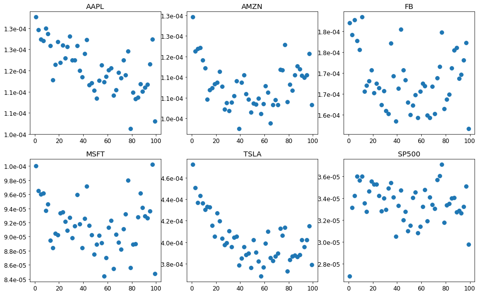
From the above plot, we choose the smallest minute after which the realized variance stablize and this corresponds to the values listed below and we can trasnform the data to get daily realized variance.
SPACING = {
    "AAPL" : 40,
    "AMZN" : 30,
    "FB"   : 10,
    "MSFT" : 10,
    "TSLA" : 40,
    "SP500": 10
}

def collapse_daily(returns, spacing=SPACING):
    RVs = multipleRVs(returns, spacing)
    returns = returns.groupby(returns.index.date).sum()
    index = pd.MultiIndex.from_product([returns.columns, ["RV", "return"] ] )
    data = pd.DataFrame(np.zeros((RVs.shape[0], RVs.shape[1]*2)),
                        index = RVs.index, columns = index)
    for j in RVs.columns:
        data.loc[:, (j,"return")] = returns[j]
        data.loc[:, (j, "RV")] = RVs[j]
    return data
train_daily = collapse_daily(train)
test_daily = collapse_daily(test)

index = (train_daily["TSLA"]["RV"] == 0)
train_daily = train_daily[~index]
train_daily
| AAPL | AMZN | FB | MSFT | TSLA | SP500 | |||||||
|---|---|---|---|---|---|---|---|---|---|---|---|---|
| RV | return | RV | return | RV | return | RV | return | RV | return | RV | return | |
| 2019-01-02 | 0.000276 | 0.018817 | 0.000566 | 0.047986 | 0.000478 | 0.044343 | 0.000252 | 0.021878 | 0.000517 | 0.012795 | 0.000143 | 0.014631 |
| 2019-01-03 | 0.000334 | -0.014916 | 0.000346 | -0.017998 | 0.000446 | -0.021329 | 0.000419 | -0.025744 | 0.000573 | -0.024370 | 0.000222 | -0.019205 |
| 2019-01-04 | 0.000240 | 0.025416 | 0.000369 | 0.031095 | 0.000224 | 0.023634 | 0.000381 | 0.025587 | 0.000389 | 0.032885 | 0.000171 | 0.022167 |
| 2019-01-07 | 0.000355 | -0.002600 | 0.000272 | 0.019787 | 0.000296 | 0.001024 | 0.000194 | 0.005699 | 0.000679 | 0.040694 | 0.000068 | 0.006271 |
| 2019-01-08 | 0.000114 | 0.007528 | 0.000419 | -0.002183 | 0.000299 | 0.012709 | 0.000191 | -0.003128 | 0.001019 | -0.021433 | 0.000087 | 0.001863 |
| ... | ... | ... | ... | ... | ... | ... | ... | ... | ... | ... | ... | ... |
| 2019-11-22 | 0.000038 | -0.002365 | 0.000027 | 0.004836 | 0.000064 | -0.000905 | 0.000034 | -0.003204 | 0.000223 | -0.020516 | 0.000007 | -0.000595 |
| 2019-11-25 | 0.000022 | 0.012085 | 0.000052 | 0.008161 | 0.000050 | 0.000200 | 0.000012 | 0.006900 | 0.000164 | -0.014727 | 0.000004 | 0.003998 |
| 2019-11-26 | 0.000012 | -0.006490 | 0.000035 | 0.009007 | 0.000034 | -0.004639 | 0.000016 | 0.003198 | 0.000120 | -0.016852 | 0.000006 | 0.002352 |
| 2019-11-27 | 0.000011 | 0.008658 | 0.000036 | 0.011019 | 0.000085 | 0.011351 | 0.000013 | 0.000722 | 0.000083 | 0.004661 | 0.000002 | 0.002683 |
| 2019-11-29 | 0.000007 | 0.001948 | 0.000030 | -0.010237 | 0.000081 | 0.001410 | 0.000015 | -0.004232 | 0.000027 | -0.000545 | 0.000003 | -0.001396 |
229 rows × 12 columns
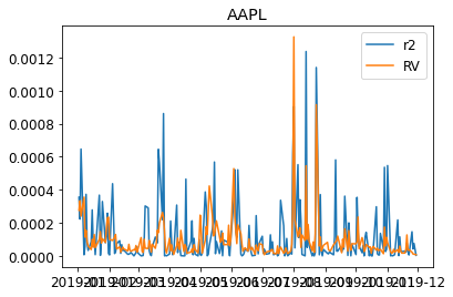
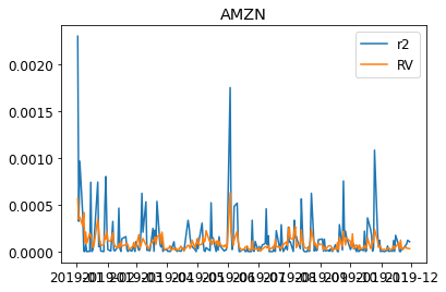
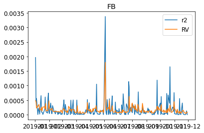
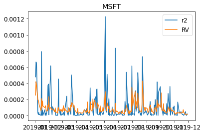
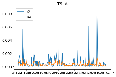
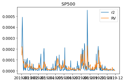
We can visualize the realized variance and the squared log returns.
for s in DATA:
    plt.figure()
    plt.title(s)
    plt.plot((train_daily[s]["return"]**2),label="r2")
    plt.plot(train_daily[s]["RV"],label="RV")
    plt.legend(loc = "best")
    plt.show()
We then fit the individual realized Garch
GARCHs = {}
PARAMs = {}
scale = 1e3
for symbol in DATA:
    print ("fit symbol "+ str(symbol) + " ...")
    returns = train_daily[symbol]["return"]
    RVs = train_daily[symbol]["RV"]
    rl_garch = RealizedGARCH(returns, RVs, scale = scale)
    rl_garch.fit(verbose = 0)
    GARCHs[symbol] = rl_garch
    params = pd.concat( (rl_garch.params, rl_garch.measure_params) )
    PARAMs[symbol] = params

PARAMs = pd.DataFrame.from_dict(PARAMs, orient="columns")
PARAMs
fit symbol AAPL ...
	 best L1 = -650.558
fit symbol AMZN ...
	 best L1 = -668.673
fit symbol FB ...
	 best L1 = -711.490
fit symbol MSFT ...
	 best L1 = -636.488
fit symbol TSLA ...
	 best L1 = -816.116
fit symbol SP500 ...
	 best L1 = -498.618
| AAPL | AMZN | FB | MSFT | TSLA | SP500 | |
|---|---|---|---|---|---|---|
| omega | 0.000035 | 0.000013 | 0.000012 | 0.000011 | 0.000241 | 0.000003 |
| beta | 0.306265 | 0.804552 | 0.932296 | 0.665771 | 0.000000 | 0.415299 |
| gamma | 0.498232 | 0.112582 | 0.000000 | 0.248973 | 0.762372 | 0.502016 |
| mu | 0.001039 | 0.000049 | 0.000246 | 0.000175 | 0.000450 | 0.000387 |
| xi | 0.221838 | 7.076395 | 153.648558 | 2.076153 | -1.130535 | -0.787398 |
| phi | 1.084924 | 1.846474 | 18.791195 | 1.256567 | 0.931592 | 0.943701 |
| tau1 | -0.101627 | -0.092318 | -0.105260 | -0.072026 | -0.026562 | -0.174259 |
| tau2 | 0.244832 | 0.176118 | 0.134127 | 0.156663 | 0.149789 | 0.153689 |
| sigmaU | 0.650246 | 0.584097 | 0.490212 | 0.444128 | 0.566098 | 0.554517 |
def realizedGarch_log_likelihood():
    Likelihoods = {}
    for symbol in GARCHs:
        Likelihoods[symbol] = GARCHs[symbol].train_log_likelihood()
    Likelihoods = pd.DataFrame.from_dict(Likelihoods, orient= "index")
    Likelihoods.columns = ["log(L)"]
    Likelihoods = Likelihoods.transpose()
    return Likelihoods

def get_garchs():
    original_garches = {}
    for symbol in DATA:
        am = arch_model(1000*train_daily[symbol]["return"], mean='Constant', vol='garch')
        res = am.fit(disp="off")
        original_garches[symbol] = res

    return original_garches

def arch_log_likelihood(arches, scale = 1):
    ans = {}
    for symbol in arches:
        arch_res = arches[symbol]
        vol = (arch_res.conditional_volatility/scale)**2
        resid = arch_res.std_resid
        loglikelihood = -0.5*np.sum(np.log(2*np.pi*vol) + resid**2)
        ans[symbol] = loglikelihood
    ans = pd.DataFrame.from_dict(ans, orient="index")
    ans.columns=["log(L)"]
    ans = ans.transpose()
    return ans
We fit our reailized Garch model and the classical Garch separately and compare them by the likelihoods. Our realized model achieves better value in AAPL, MSF, TSLA and SP500. The fit for AMZN and FB seems not working.
realizedGarch_log_likelihood()
| AAPL | AMZN | FB | MSFT | TSLA | SP500 | |
|---|---|---|---|---|---|---|
| log(L) | 720.881208 | 702.766017 | 659.948803 | 734.951069 | 555.322595 | 872.821334 |
arch_log_likelihood(get_garchs(), scale = 1000)
| AAPL | AMZN | FB | MSFT | TSLA | SP500 | |
|---|---|---|---|---|---|---|
| log(L) | 714.535985 | 708.639553 | 662.078304 | 734.394404 | 549.42429 | 867.143143 |
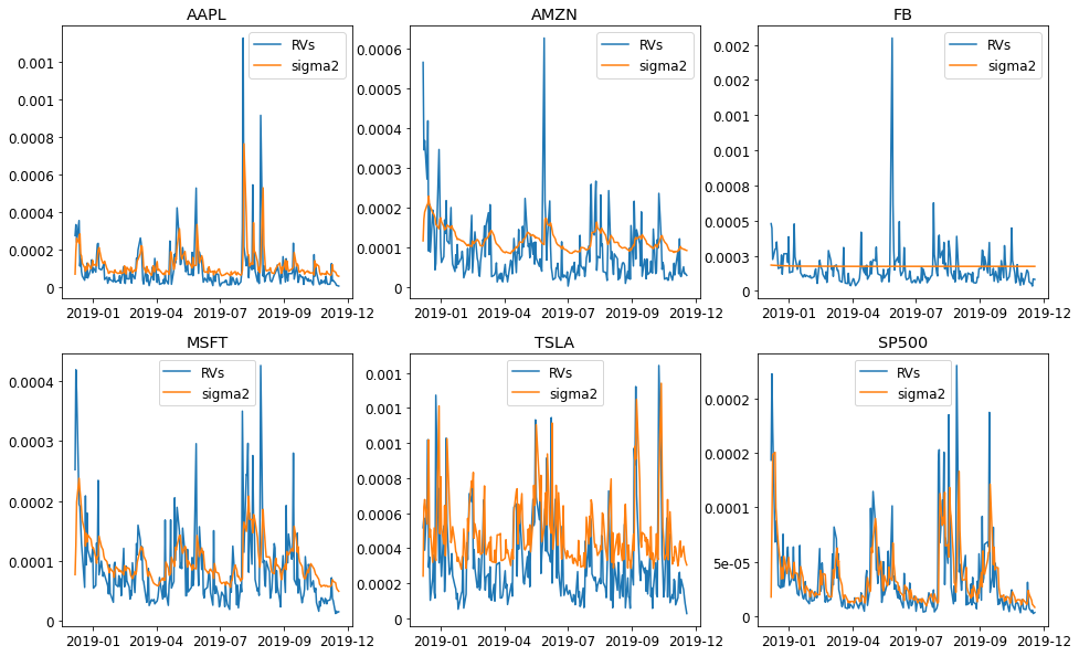
From the below plot its clear why the FB and AMZN do not show higher likelihood. The fitted conditional variance $\sigma^2$ doest follow the realized variance. Especially, the FB model has $\beta = 0$ and does not take into account of realized variance in the model. The AMZN has very small coefficient for $\beta$ and is thus very insensitive to the change of the market (the rise or fall of realized variance).
fig, axs = plt.subplots(2, 3, figsize=(16,10))
for i in range(2):
    for j in range(3):
        ax = axs[i][j]
        symbol = RV_tuning.columns[i*3+j]
        GARCHs[symbol].plot(ax= ax)
        ax.xaxis.set_major_locator(MaxNLocator(5))
        ax.xaxis.set_major_formatter(mdates.DateFormatter("%Y-%m"))
        ax.xaxis.set_minor_formatter(mdates.DateFormatter("%Y-%m"))
        ax.yaxis.set_major_formatter(FormatStrFormatter('%1.1g'))
        ax.title.set_text(symbol)
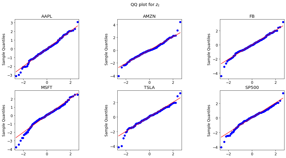
def plot_z(Garchs):
fig, axs = plt.subplots(nrows=2, ncols=3, figsize=(16,8))
fig.suptitle(r"QQ plot for $z_t$")
plt.subplots_adjust(wspace = 0.6)
axs = axs.reshape(-1)
for j, stock in enumerate(Garchs):
ax1 = axs[j]
ax1.set_title(stock)
qqplot(Garchs[stock].std(), line = "s", ax = ax1)
ax1.set_xlabel("")
plt.savefig("zt.png")
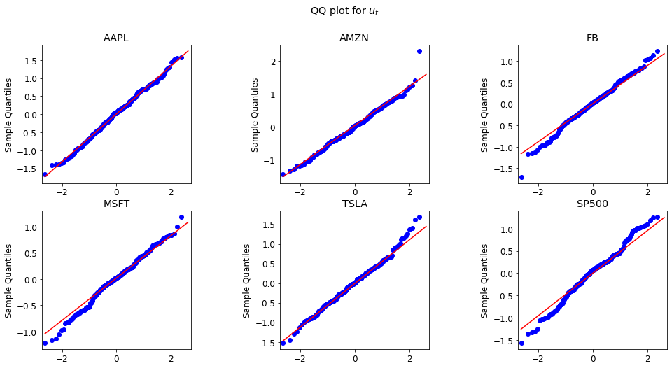
def plot_u(Garchs):
fig, axs = plt.subplots(nrows=2, ncols=3, figsize=(16,8))
fig.suptitle(r"QQ plot for $u_t$")
plt.subplots_adjust(wspace = 0.6)
axs = axs.reshape(-1)
for j, stock in enumerate(Garchs):
ax1 = axs[j]
ax1.set_title(stock)
measure_RV = Garchs[stock].measure_RV()
diff = np.log(measure_RV) - np.log(Garchs[stock].RVs_original[1:])
qqplot(diff, line = "q", ax = ax1)
ax1.set_xlabel("")
plt.savefig("ut.png")
We plot fitted residual for $z_t$ and measurement linear regression residual $u_t$ in qq plot. The plot shows that they almost follow the normal distribution. As a result, the assumption is mildly satisfied.
plot_z(GARCHs)
plot_u(GARCHs)
DCC correlations
We fit the rGARCH-DCC model with the DCC employed to describe the correlation among the shocks $z_t$ among the symbols.
rGarch = RGARCH_DCC(train_daily, garch_scale = 1000)
rGarch.fit(verbose = 0)
rGarch.params()
fit AAPL ...
	 best L1 = -650.558
fit AMZN ...
	 best L1 = -668.673
fit FB ...
	 best L1 = -711.490
fit MSFT ...
	 best L1 = -636.488
fit TSLA ...
	 best L1 = -816.116
fit SP500 ...
	 best L1 = -498.618
iteration: 1 	 log(L): 73.840 	 a: 0.38595 	 b:0.61405
iteration: 2 	 log(L): 680.975 	 a: 0.3732 	 b:0.31926
iteration: 3 	 log(L): 672.804 	 a: 0.3509 	 b:0.58848
iteration: 4 	 log(L): 515.326 	 a: 0.31236 	 b:0.68764
iteration: 5 	 log(L): 543.880 	 a: 0.30289 	 b:0.69711
iteration: 6 	 log(L): 579.609 	 a: 0.2883 	 b:0.7117
iteration: 7 	 log(L): 572.286 	 a: 0.29162 	 b:0.70838
iteration: 8 	 log(L): 625.487 	 a: 0.25989 	 b:0.74011
iteration: 9 	 log(L): 533.779 	 a: 0.30642 	 b:0.69358
iteration: 10 	 log(L): 649.872 	 a: 0.19871 	 b:0.80129
iteration: 11 	 log(L): 687.172 	 a: 0.30417 	 b:0.62254
iteration: 12 	 log(L): 687.863 	 a: 0.30861 	 b:0.59438
iteration: 13 	 log(L): 687.865 	 a: 0.30947 	 b:0.59154
iteration: 14 	 log(L): 687.865 	 a: 0.30952 	 b:0.59176
iteration: 15 	 log(L): 687.865 	 a: 0.30948 	 b:0.59181
iteration: 16 	 log(L): 687.865 	 a: 0.30948 	 b:0.59181
rGarch parameters:
            AAPL      AMZN          FB      MSFT      TSLA     SP500
omega   0.000035  0.000013    0.000012  0.000011  0.000241  0.000003
beta    0.306265  0.804552    0.932296  0.665771  0.000000  0.415299
gamma   0.498232  0.112582    0.000000  0.248973  0.762372  0.502016
mu      0.001039  0.000049    0.000246  0.000175  0.000450  0.000387
xi      0.221838  7.076395  153.648558  2.076153 -1.130535 -0.787398
phi     1.084924  1.846474   18.791195  1.256567  0.931592  0.943701
tau1   -0.101627 -0.092318   -0.105260 -0.072026 -0.026562 -0.174259
tau2    0.244832  0.176118    0.134127  0.156663  0.149789  0.153689
sigmaU  0.650246  0.584097    0.490212  0.444128  0.566098  0.554517

DCC parameters:
a    0.309478
b    0.591807
dtype: float64
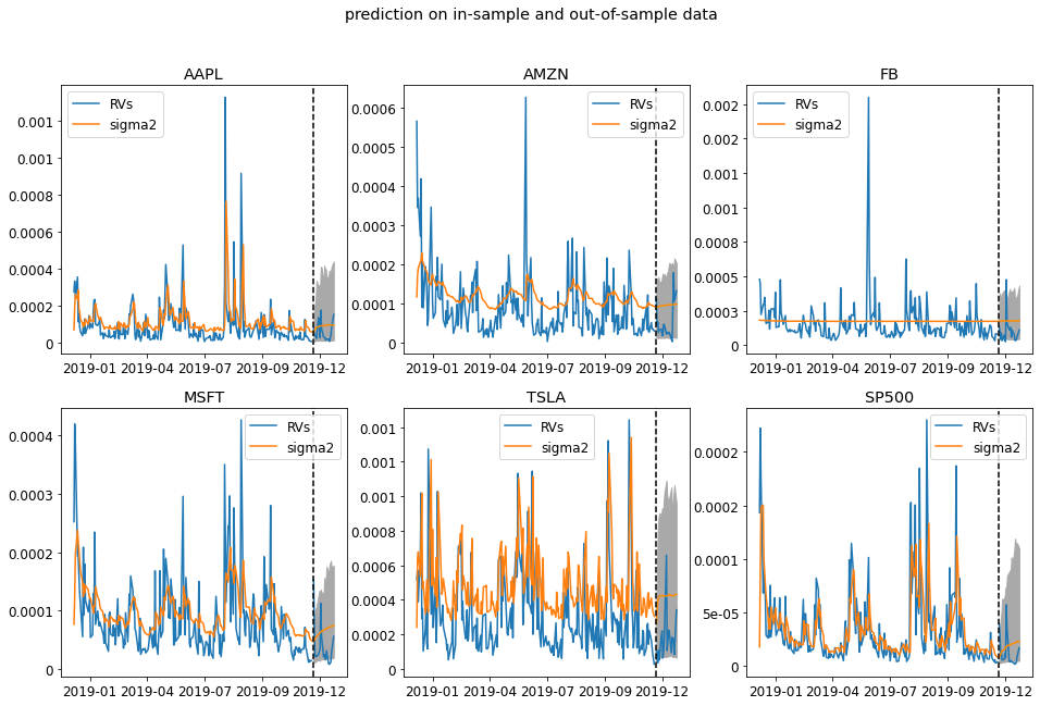
def plot_predict(RGARCH, test, n_sample = 1000, low_q = 0.025, high_q = 0.975):
    horizon = test.shape[0]
    sigma2_pred, RV_pred = RGARCH.predict_horizon(
                                horizon,
                                n_sample = n_sample,
                                low_q = low_q, high_q = high_q)
    sigma2_mean = pd.DataFrame(sigma2_pred[1,...])
    sigma2_high = pd.DataFrame(RV_pred[2,...])
    sigma2_low  = pd.DataFrame(RV_pred[0,...])

    sigma2_mean.index = test.index
    sigma2_high.index = test.index
    sigma2_low.index  = test.index

    fig, axs = plt.subplots(2, 3, figsize=(16,10))
    fig.suptitle("prediction on in-sample and out-of-sample data")

    axs = axs.reshape(-1)

    for j, stock in enumerate(RGARCH.stocks):
        test_returns = test[stock]["RV"]
        ax = axs[j]
        RGARCH.GARCHs[stock].plot(ax=ax)
        ax.plot(test_returns, color ='#1f77b4')
        ax.plot(sigma2_mean.iloc[:,j], color = "darkorange")
        ax.fill_between(sigma2_mean.index, sigma2_low.iloc[:,j],
                sigma2_high.iloc[:,j], color = "darkgrey")
        ax.axvline(x=test.index[0], color = "k", linestyle = '--')
        ax.xaxis.set_major_locator(MaxNLocator(5))
        ax.xaxis.set_major_formatter(mdates.DateFormatter("%Y-%m"))
        ax.xaxis.set_minor_formatter(mdates.DateFormatter("%Y-%m"))
        ax.yaxis.set_major_formatter(FormatStrFormatter('%1.1g'))
        ax.title.set_text(stock)
    return fig
In this plot, we plot the fitted $\sigma^2$ and the predicted $\sigma^2$ in December. The gray area is the $95\%$ confidence interval for the realized variance. The plots shows that the predicted realized variance confidence interval contains the true hidden test data. This indicates a successful forecast.
fig = plot_predict(rGarch, test_daily)
fig.savefig("train_test.png")
We design a function that could use rolling bootstrap to estimate the confidence interval of the estimated parameters.
def rolling_bootstrap(train, n_bootstrap):
    length = train.shape[0] - n_bootstrap + 1
    GARCH_params = None
    DCC_params = None
    count = 0
    for i in range(n_bootstrap):
        garchDCC = RGARCH_DCC(train.iloc[i:i+length,:],
                              garch_scale = 1000)
        garchDCC.fit(verbose = 0)
        if GARCH_params is None:
            shape = [n_bootstrap] + list(garchDCC.GARCH_PARAMs.shape)
            GARCH_params = np.zeros(shape=shape)
        if DCC_params is None:
            DCC_params = np.zeros(shape = (n_bootstrap, 2))
        if garchDCC.DCC_PARAMs["b"] <= 1.0e-5 :
            continue
        GARCH_params[i,:,:] = garchDCC.GARCH_PARAMs
        DCC_params[count,:] = garchDCC.DCC_PARAMs
        count +=1

    GARCH_params_std = np.std(GARCH_params, axis = 0)
    DCC_params_std = np.std(DCC_params[:count,:], axis = 0)

    GARCH_params_std = pd.DataFrame(GARCH_params_std)
    GARCH_params_std.index = garchDCC.GARCH_PARAMs.index
    GARCH_params_std.columns = garchDCC.GARCH_PARAMs.columns

    DCC_params_std = pd.Series(DCC_params_std)
    DCC_params_std.index = garchDCC.DCC_PARAMs.index
    print (count)
    return GARCH_params_std, DCC_params_std
rGarch.GARCH_PARAMs
| AAPL | AMZN | FB | MSFT | TSLA | SP500 | |
|---|---|---|---|---|---|---|
| omega | 0.000035 | 0.000013 | 0.000012 | 0.000011 | 0.000241 | 0.000003 |
| beta | 0.306265 | 0.804552 | 0.932296 | 0.665771 | 0.000000 | 0.415299 |
| gamma | 0.498232 | 0.112582 | 0.000000 | 0.248973 | 0.762372 | 0.502016 |
| mu | 0.001039 | 0.000049 | 0.000246 | 0.000175 | 0.000450 | 0.000387 |
| xi | 0.221838 | 7.076395 | 153.648558 | 2.076153 | -1.130535 | -0.787398 |
| phi | 1.084924 | 1.846474 | 18.791195 | 1.256567 | 0.931592 | 0.943701 |
| tau1 | -0.101627 | -0.092318 | -0.105260 | -0.072026 | -0.026562 | -0.174259 |
| tau2 | 0.244832 | 0.176118 | 0.134127 | 0.156663 | 0.149789 | 0.153689 |
| sigmaU | 0.650246 | 0.584097 | 0.490212 | 0.444128 | 0.566098 | 0.554517 |
rGarch.DCC_PARAMs
a    0.309478
b    0.591807
dtype: float64
def getRV_data(data, weights):
indexs = data.columns.get_level_values(0).unique()
returns = np.zeros( (data.shape[0], len(indexs)) )
for i,symbol in enumerate(indexs):
returns[:,i] = data[symbol]["return"]
sigma2 = returns.dot(weights)**2
sigma2 = pd.Series(sigma2)
sigma2.index = data.index
return sigma2
def plot_portfolio_RV(train, test, model, weights, low_q = 0.025,
high_q = 0.975, ax = None):
model_sigma2 = model.get_portfolio_sigma2(weights)
train_sigma2 = getRV_data(train_daily, weights)
test_sigma2 = getRV_data(test_daily, weights)
pred_sigma2 = rGarch.predict_horizon_portfolio(
test_sigma2.shape[0],
weights,
low_q = low_q, high_q = high_q)
pred_sigma2 = pd.DataFrame(pred_sigma2.T)
pred_sigma2.index = test_daily.index
if ax is None:
ax = plt.gca()
ax.plot(train_sigma2, color = "#1f77b4", label = r"$r^2$")
ax.plot(test_sigma2, color = "#1f77b4")
ax.plot(model_sigma2, color = "darkorange", label = r"model $\sigma^2$")
ax.plot(pred_sigma2.iloc[:,1], color = "darkorange")
ax.fill_between(pred_sigma2.index, pred_sigma2.iloc[:,0],
pred_sigma2.iloc[:,2], color = "darkgrey")
ax.axvline(x=test.index[0], color = "k", linestyle = '--')
ax.legend(loc="best")
return
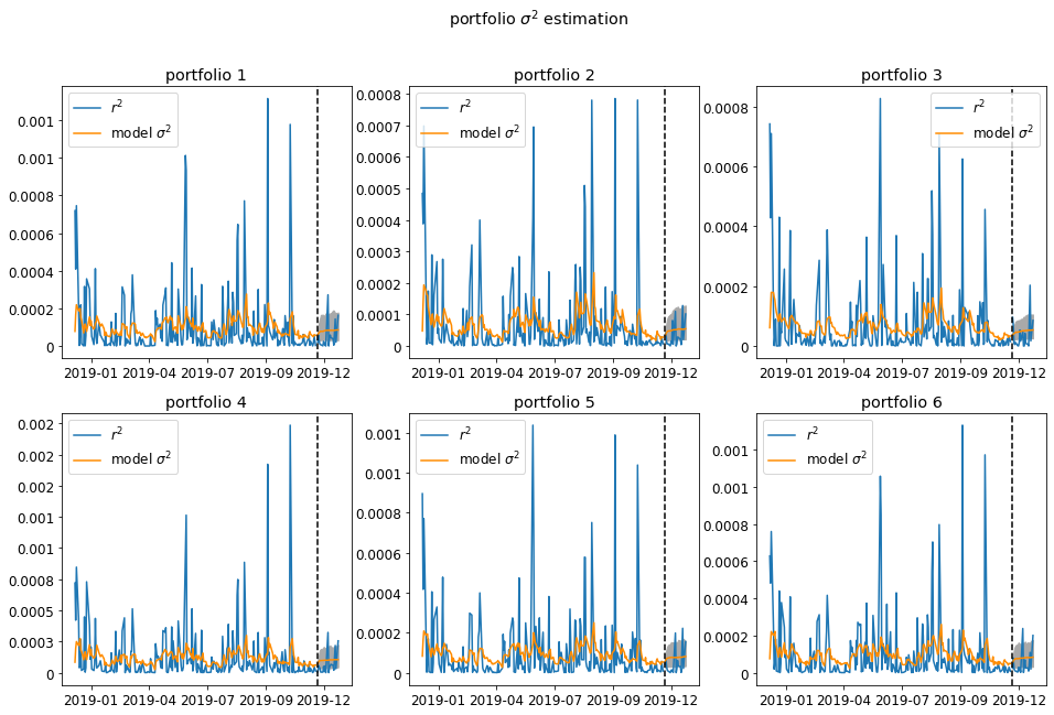
def plot_six_pack(train, test, model, weights = None,
low_q = 0.025, high_q = 0.975):
symbols = train.columns.get_level_values(0).unique()
n_symbols = len(symbols)
if weights is None:
weights = np.random.uniform(size=(6, n_symbols))
weights = weights/np.sum(weights, axis=1)[:,None]
fig, axs = plt.subplots(2, 3, figsize=(16,10))
fig.suptitle(r"portfolio $\sigma^2$ estimation")
print (weights)
print (weights.sum(axis=1))
axs = axs.reshape(-1)
for i in range(6):
ax = axs[i]
plot_portfolio_RV(train, test, model, weights[i,:],
low_q, high_q, ax = ax)
ax.xaxis.set_major_locator(MaxNLocator(5))
ax.xaxis.set_major_formatter(mdates.DateFormatter("%Y-%m"))
ax.xaxis.set_minor_formatter(mdates.DateFormatter("%Y-%m"))
ax.yaxis.set_major_formatter(FormatStrFormatter('%1.1g'))
ax.title.set_text(f"portfolio {i+1:d}")
return fig
We then construct six random portfolio consisting of the 6 symbols we have. We do this because we want to test whether the correlation matrix is estimated well. The portfolio volatility needs the correlation matrix and individual volatility. Below we plotted the fitted portfolio $\sigma^2$ and the prected $\sigma^2$ in December. The blue line is the portfolio realized return squared.
fig = plot_six_pack(train_daily, test_daily, rGarch)
plt.savefig("six_pack.png")
[[0.16405074 0.17298219 0.19924118 0.0351977  0.247057   0.18147119]
 [0.12837752 0.19303799 0.01225164 0.04758079 0.17934214 0.43940992]
 [0.10489163 0.25960325 0.0583599  0.26450911 0.0773851  0.23525101]
 [0.09721203 0.31495958 0.05358826 0.04046787 0.3348108  0.15896146]
 [0.14997454 0.26229132 0.18209948 0.11644926 0.19562806 0.09355733]
 [0.0638383  0.15728596 0.12019817 0.25126211 0.2573531  0.15006237]]
[1. 1. 1. 1. 1. 1.]
Leave a comment